
Data Science 101
My story of exploring and analyzing data and trying to build a robust pipeline with classification task on my hands, having almost 0 experience in data science

Background
I have a statistical background, though never in my life, I’ve worked with statistics. I got rusty; I mean, short fragments exist about what is MSE, AUC, etc., but that is it. I have to start almost from 0 if I’d want to progress further (statistical courses I took in University were 10 years ago).
I work as a data developer/engineer by day and father of two 24/7. Whenever I have free time from these activities, I try to do something interesting to me. I had a data science field for some time in my backlog, but I couldn’t find a good use case to deep dive into it. The Focus area for me (is now) and was stream processing, Apache Spark, and other Big Data processing related things.
Keep in mind that this is the first legit time I tried to make some predictions. I’m not doing anything production-grade, and this post is most likely to be useful for new kids on the Data Science block (explorers or just starting). Learn from my mistakes as well!
To emphasize: I’m not connected with any of the vendors, libraries I mentioned. All is done and written based on my personal experience and point of view!
Generics of Data Science
Data Science has a lifecycle, by following which we can do things in an orderly fashion.
I imagined it something like
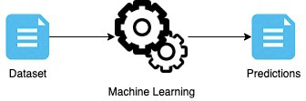
Machine Learning part being model.fit(X,y) and model.predict(Z). But oh boy, how was I wrong. I was missing a lot of steps in the middle.
We have:
Data exploration
Data preprocessing
Machine Learning
Data Exploration
I imagine most of the cases or at least play around happen with the Pandas library. All my examples and code snippets will be made with the Pandas data frame.
First rule of data science is that we explore data first!
At least, this is what I imagine. Data exploration may unravel all the issues you have, which you can resolve and make your life way easier.
A bit about the dataset I had — it was used in some local competition, and it simplified looked like this:

Mistake number 1 — No data exploration.
Please, don’t stop reading now, I encountered a million issues, and my ML model was doing coin flip accuracy. After that, I’ve started investigating my data.
Describe
Though originally, I didn’t try to look at this method until my colleague shared its value. Describe provides the most generic information, from which we can see our data skewness, outline potential outliers in some columns.

If we see huge differences in percentile values, we might have issues to solve. In the image above, we can see that our column amount_current_loan has a max value of 99999999, which is ~200 times bigger than 75%. However, the column doesn’t have missing values. I naturally implied that a particular constant is a result of treating missing values. Already one issue solved by one quick glimpse at the summary table.
Missing values
By using simple pandas expression
data.isna().sum()we get a good image of how many values we have missing and focus on the data preprocessing step.
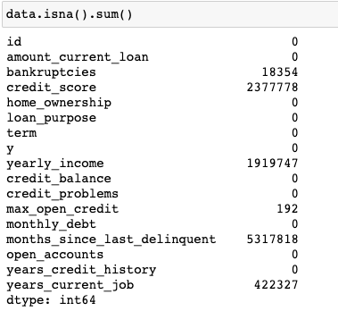
We’ll get to this information's usefulness in Part 2 and how to deal with this issue.
Correlation
A good thing to check upon is the correlation between our columns. Pandas have a method which does it quite easily:
data.corr()it will provide a data frame back as a result

We have to check on numbers row by row, and it gets out of hand fast. Maybe we can plot this and have a more visually pleasing approach? As with Python — we have libraries for everything. This is not an exception. I knew about matplotlib before, but as I recalled, it required a bit of tinkering; I was 99% sure that there is a library for easier use. In this case, it was Seaborn. Easy to use and graphically pleasing. And for correlation best thing is a heatmap.
Seaborn has a heatmap method. It has lots of customizations, though for everything to be properly readable, I had to google some things out and use matplotlib.
import seaborn as sns
import matplotlib.pyplot as pltfig, ax = plt.subplots(figsize=(10,10))
sns.heatmap(data.corr(), vmin=-1, vmax=1, annot = True, ax=ax, fmt=".2f")
Though I like the output - formatted, readable, and you can see what’s correlating and what level in between columns.

You can check out seaborn documentation for more information about the parameters I’ve passed.
So from the heatmap, we can see that only two columns have a high correlation (by high — I mean 0.7+). It’s credit_problems with bankruptcies, which is obvious if you think about it. What is great (not sure if I can categorize it like this), that I have NaN values in the bankruptcies column and no missing values in the credit_score. I can use one to infer other missing values. Keep an eye on this in Part 2.
Outliers
These pesky critters can cause tons of issues on your model. They will mess with your loss function and will result in poor accuracy. We need to treat them somehow.
Another amazing visualization comes to play — seaborn.boxplot.
import seaborn as sns
sns.boxplot(x=data["yearly_income"])
In a couple of iterations filtering on values, we end up with data clean from outliers:
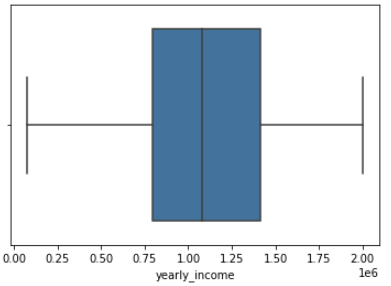
Free of some of the biggest outliers at last!
Distribution
Ok, so let’s check what distribution our column values has.
sns.displot(data["years_credit_history"])
Investigating it visually (there are some light blue lines), we see that it looks like the normal distribution, but it’s skewed to the left. There is a solution to it! Let’s use np.log1p on column and see if it solves the issue:
sns.displot(np.log1p(df["years_credit_history"]))
If you’re not familiar with how normal distribution looks like:

Preprocessing
Initial steps
The usual approach is to do the manipulations in pandas then apply the same ones on the prediction dataset. I.e., do One Hot Encoding (with dummies)
dum_df = pd.get_dummies(df["credit_score"], columns=["credit_score"], prefix="credit_score")
df = df.join(dum_df).drop("credit_score", axis=1)
so for playing around until you get steps sorted out — it’s straightforward. Though working on some ML things (the challenge which got me hooked on DS) and mostly working in Jupyter Notebooks, It’s easy to get lost. Also, it’s hard to track all the changes (and current data values). This won’t work in production pipelines; even slight changes might mess the pipeline!
Transformers
Transformers are helper functions that ease your life, maintaining and quickly adding new transformations on your data fast and in a testable way!
Most of the transformation already exists in sklearn!
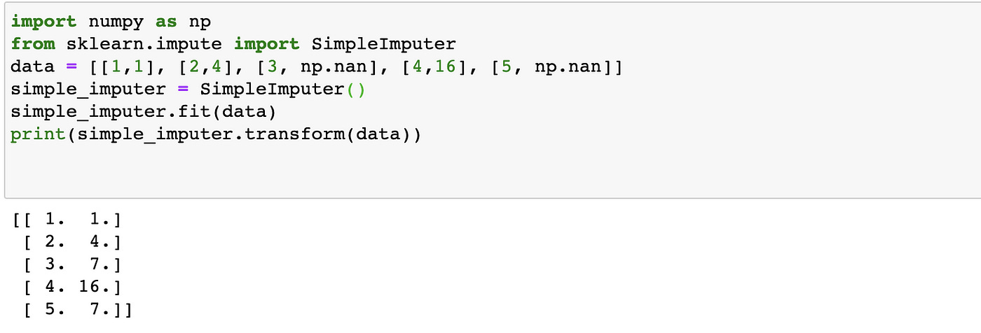
SimpleImputer
Remember my NaN issues? We can use this Imputer to fill missing values, which can be NaN or any other different value we specify, to the values we want. The default strategy is mean, but we can use the median, most_frequent, and constant.
Spark Analogy Imputer
Dask Simple Imputer
IterativeImputer
Let’s say we want a bit more intelligent imputation. We can use (still experimental, though) — IterativeImputer. Which comes way close than it should [3, 9], [5,25] was expected. Compared to simple mean/median, which wouldn’t be sufficient here.

You can choose a different estimator, which might lead to a better imputation:

It only exists on sklearn!
OneHotEncoder
First thing first about encoders. Encoders after fit can be easily used to transform your prediction dataset without any worries. All the logic will be the same as in the dataset you trained it with. Though you didn’t have any value in the fitted dataset, you can probably use some parameters to handle it. It’s more robust and customizable than doing some transformations on your own.
Let’s talk about this OneHotEncoder in particular. It creates multiple columns based on values of it. There is a param on handling unknown values: handle_unknown{‘error,’ ‘ignore’}

We can also drop one of the new columns per category to avoid a perfect correlation using the drop parameter!
Alternatives in other libraries: Spark, Dask
StandardScaler
Basically, it subtracts the mean of the column and divides by variance. The cool thing is that once you create a scaler, you can re-use it on other columns/data frames as long as it’s logically ok.

One issue with it, if you have outliers, your data will look not that great:
This functionality exists in Dask, Spark.
RobustScaler
This bad boy here helps to solve this issue:
Our initial values are more or less similar if we had them without the outlier. Data is more standardized more properly, but we’ll have to take care of the outlier later!
Pipeline
Its name says everything about it. Pipeline of actions you want to execute. It can be combined from transformers and then model fitting. It is handy to ensure your model will be treated in the same way and have exact steps in it.

Alternatives in other libraries: Dask uses sklearn, Spark
ColumnTransformer
Ok, so this was really a new thing for me. Apparently, using this transformer, you can specify steps to be executed on particular columns.

One of the transformers is to impute NaN values to be filled with constant “missing” and the OneHotEncode.

You can write your own transformer to keep it in the same manner as existing ones, i.e., fill NaNs with median/mean/mode per group, reduce cardinality based on threshold, and many others. Most of your transformations can probably be made in the same format.
It doesn’t support my needs! I will use my transformations.
Though it may look that only basics are covered, there is a way to add your own transformers.
You create a new object in python. In my case, I had several custom transformations. One was filling bankruptcies based on credit_problems with most_frequent value. Another was cardinality reducer:
It’s not that robust, I could make it more generic and tunable, but it satisfied my needs.
I used it on several categorical numerical columns and merged all small groups into one.
I passed a list of groups, and it bucketed them the way I intended to.
All in all, you can make a concrete (and robust!) pipeline by combining pipeline with column transformers. All of your custom transformers can be tested separately before introducing them to your production pipeline and ensure that it’s pipeline compatible. Though after testing it thoroughly, you will be sure it will not break anything!
Data Imbalance — imblearn
The first prediction resulted in 10k rows of 0s. I was surprised. Why it went like this? Did none of them have some features to become 1? Then I investigated the distribution of labels:

So we have a ratio of 3:1. This probably happened because the train test model’s random split was not done properly (not keeping the ratios or something similar).
We have several options here:
splitting the train test, we use the stratify option.
Make our dataset split more evenly.
So let’s go with the latter one. At first, I manually extracted the minority class and repeated it until we have a more or less similar count. I noticed that it’s not efficient. If I try to do it per one dimension value, I quickly get lost. As usual with python, I thought there has to be a library for this.
And apparently there was! Library imblearn is dedicated to help you solve this issue! You can choose different methods of oversampling, under-sampling, or even a combination of them.
The bonus part of it they have an ensemble part for models, which solves imbalance!

Flow will not change since we can use imblearn Pipeline:
from imblearn.pipeline import PipelineWith minor changes in the code (instead of sklearn, use imblearn), we can use any imbalance-fixing technique.
Power of pipeline!
Now your data preparation will be robust, and you will be sure that your train dataset and the one you’ll be basing your predictions will follow the same manipulations in the same order!
Classification
Since the challenge this post is based on was classification type, I will cover only classification here.
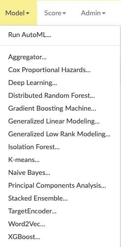
The most common (or at least it was for me) understanding that sklearn is the most used library for ML. Before going to baseline results, I’m going to present some of the libraries. Keep in mind I’m aiming here at fresh Data Scientist or this path explorers, so I’m not going to Neural Network libraries (Keras, Tensorflow, PyTorch).
Disclosure
I didn’t invest time in this challenge when it was ongoing of being too busy with other things. I still managed to get a 0.78 AUC score, which is not that bad to my newcomers' eyes. From my point of view, it’s not that bad for a rookie. The biggest mistake I’ve made — not logging my models, parameters properly could have made my life easier when I would fine-tune them. I didn’t know many different techniques as Stacking, Voting, which I could have used to my advantage as well for Catboost and LightGBM, which had pretty high accuracy. I’ll overview what I could have done better (or used it to my advantage), not going into the modeling itself.
MLFlow
MLflow — A platform for the machine learning lifecycle
An open-source platform for the machine learning lifecycle MLflow is an open-source platform to manage the ML…
How many times you ran a model, got a good score, but the next day you couldn’t reproduce because you’ve made some changes here and there (different configuration, dataset)? At least to me, it was getting out of hand quite fast. Only printing some configuration, and the AUC score was getting lost pretty fast. I needed to track all of the configurations, scores, and data in general somehow. Using this platform, I could have logged my best model and then fine-tune it. Best discovery for me, though it was a bit too late for the challenge.
H2O
This one is a library for doing ML, similar to sklearn. Though it has UI, on which you can do your ML by clicking multiple mouse buttons. Import data, explore it, impute missing data if you’d like, and then even run AutoML, which will search on models and configuration to find the best one (also stacks them at the end!). I’d say it can help even a person having almost none programming experience to do ML.

If you want more customization, it has python and R API for you to interact with.
I was not too fond of that H2OFrame doesn’t quite work like pandas/spark/dask data frames sometimes. It was a bit hard to figure out how to do certain things, i.e., get a list of distinct column values. Here I had to use flatten, though in pandas would be list(). Nonetheless pretty cool library which can help anyone!
PyCarret
Another amazing library that I found, though I couldn’t make it work on this dataset. I think I was just impatient with its long search for hyperparameter tuning.
This snippet would fix imbalances, remove outliers and fit multiple models with a search on hyperparameters. My data was around 1GB CSV file, so even 5 folds take some time on one model. Keeping in mind that there is hyperparameter tunning + multiple models + 5 folds = too long waiting time. If I’d have smaller datasets, I’d definitely give it a try again; it seems easy to work with, and it does all the work for you!
FastAI
I remember trying to play with TensorFlow a couple of years ago for some face recognition and then train the model to get the person's name. I remember, in general, creating a convolutional neural network quite complicated for that non-experienced person. Then I moved on and just recently started seeing FastAI being on the hype, so it came as one possible model when I started this challenge.
Their framework is easy to work with, specifying layers similar to MLPClassifier in sklearn — pass a list with neuron count in each layer. Though running your training on CPU will drive you mad (it takes A LOT of time, like literally A LOT). In my case, when I used the CPU, it showed 150+ hours. None of my owned machines had an Nvidia GPU inside, so it wasn’t on my list to try first. In later parts, I’ll tell how to use free GPU on some platforms and speed up any model training that can leverage GPU.
Hyperparameter tuning
Let’s do a hyperparameter tuning for them. Usual helpers are GridSearchCV (exhaustive search) or RandomSearchCV (not necessarily get the best combination) from sklearn. I was so glad that I found out about this amazing gem — scikit-optimize. It has BayesSearchCV. It takes ranges and takes a parameter of several iterations. It should try to optimize your model based on the scorer you provide. Minor issue with this that it could fall to a local minimum, and you wouldn’t improve anywhere.
Small sneak peek on how some models performed to OverSampling and BayesSearchCV hyperparameter tuning:

Keep in mind over sampling is not always leading to more accurate results. Maybe your data is at exact split it has to be?
Platforms with GPU
Google Colaboratory
Amazing platform where you can do ML without using any of your resources. All works on a prettier jupyter notebook environment (at least for me).
There are several options for hardware acceleration:
None — using CPU

GPU — with Nvidia card (these I’ve personally have gotten in different notebooks T4, K80, P100)
TPU — Tensor processing unit, aimed at increasing TensorFlow performance
Since this machine can crash, etc., my suggestion is to put your data to your google drive and then mount it and access files from it:
and access your data in the usual way, just from /content/drive. Though I guess you agree with google seeing your data, which might not work for sensitive information. Though for Kaggle and playing around, it works quite well.
Another way is to store your data somewhere and pull it from the internet.
Beware of some limitations. Collaboratory was designed for people to test some things, get familiar and share at ease. So probably, you won’t be able to run long pipelines on the free version. This version gives 12h of being connected (after that, you can’t use GPU). Also, it timeouts after 90mins of nothing being pressed, basically disrupting complex, long-running neural nets or computations; you have to click some things here and there to avoid it).
There is a less restrictive Google Collab Pro; it’s 9.99$ per month. Unfortunately, it’s available only in the USA and Canada.
BlazingSQL
BlazingSQL Notebooks
Edit description
This one is aimed to let you run flows using RAPIDS. You can leverage GPUs and install any additional libraries you need. The interface is Jupyter Hub. Honestly, I somehow liked Colab more than BlazingSQL. It’s a good alternative to do the same GPU accelerated computation as well. You can mount the same google drive if you want, but if you’d upload your files here, it would stay there even if your server is restarted, not like in Colab.
Summary
I’ve covered how to explore and analyze your data using seaborn library, how to spot outliers and how to clean your data. Though keep in mind each machine learning task is different, and it might. Next, we checked several scikit-learn transformers and how they stack up and process your data. Following with, data class imbalance issues with imblearn library and some libraries I played around with. Added some tools and platforms which might make your life easier tracking your model performance or training them on GPUs (if they have this option).
Like I said, I did this out of curiosity; my submission to the task was not the best of what I could have achieved (only 0.78 AUC). If you wouldn’t make the same mistakes as I did, it will benefit you as well as it did for me.